In my previous post I addressed how to produce a view of many concordance plots at once, and presented concordance plots for twelve vocatives which are indicative of social class in Shakespeare and a larger reference corpus of Early Modern Drama.

After double-checking all the concordance plot files using a hand-numbered master sheet, I normalised the files using the command convert plot*.jpg -size 415x47! plot*.jpg (on the off chance that any files weren’t ultimately the same size), created a new folder of the normalised files, and pulled out the examples which matched the numbers I had for Shakespeare’s plays for further analysis. I hadn’t addressed titles, as I wasn’t really aiming to look at individual authors, so each file is named plot1, plot2, plot234, etc. I went on to compile the results for these plays, felt confident about the fact that I had isolated Shakespeare, and wrote up my previous blog post.

This morning I had a nagging thought: What if those weren’t Shakespeare’s plays? After all, I had broken my #1 rule about using computational methods – assuming that everything at every step of the process worked the way I thought it did. I am probably a self-parodying pendant when it comes to computational methods, because when something goes wrong at some stage in the coding process it may *never* be visible or even noticed in the final output, and this gives me reason to seriously distrust automated processes for analysis.

Ultimately, I decided I would double-check the plays I had deemed to be “Shakespeare”’s. Even though I hadn’t done much automated processing with the image files, I had assumed that the normalisation process would only change the file names to represent a modified version: so that plot10 would become plot0-10, plot 11 would become plot0-11, plot234 would become plot0-234. I had assumed the information in these files wouldn’t change, and the names would correspond to the original files.

This was not true. Instead, I had isolated a very nice sample of 36 plays which I thought matched Shakespeare’s plays in numbering, but turned out to be sampled from throughout the corpus. Matching the sampled “Shakespeare” concordance plots to the master document of concordance plots, I found that I had at least one Middleton play and at least one Seneca play in addition to some (but not all) Shakespeare plays.[1] At this point I was worried, so I re-created Shakespeare’s concordance plots from the master document of concordance plots. By redoing the concordance plots, I could guarantee that these were at least all Shakespeare’s plays in the first instance. Then I normalised them again for size, and went back to see what happens in that process. The first files were a perfect match, as I had hoped. But once I moved to the second concordance plot, I was in trouble.

Below is an image showing the unmodified concordance plot for The Taming of the Shrew (shx2), outlined in red and on the top left-hand side.The other eight concordance plots in this image are normalised for size, and even without great detail you can tell that none of these match the original file. You don’t even need to see the whole image to see this:

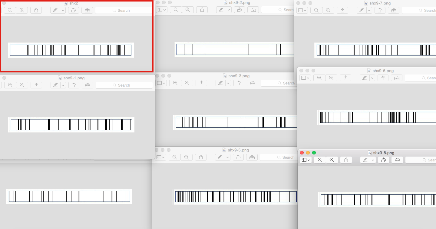
In other words, as I had suspected, the names of the normalised files didn’t correspond to the original file names, though they were all there.[2] More worryingly, I hadn’t caught it because I had assumed that the files were fine after running a process on them. The files produced results, and if I hadn’t double-checked (really, at this point, triple-checked), I wouldn’t have caught this discrepancy.

So what do concordance plots for Shakespeare’s plays look like in composite for the vocatives attached to a name in a bigram (reminder of search terms: lord [A-Z]|sir [A-Z]|master [A-Z]|duke [A-Z]|earl [A-Z]|king [A-Z]|signior [A-Z]|lady [A-Z]|mistress [A-Z]|madam [A-Z]|queen [A-Z]|dame [A-Z]) look like? Well, surprisingly, not so different from the sample curated previously, which may be less indicative of a specific authorial style:

Remember, we read these from left to right; now there’s a lot of use of vocatives in the very beginning of the plays, which stay quite strong near the rising action until there’s a relative absence just before and around the climax and the start of the falling action. Curiously, the heavy double hit || towards the end is still very visible, as well as a few more dark lines leading up to the conclusion. In some ways, the absence of these vocatives is almost more consistent, and therefore the white bits are more visible.

In the meantime I’m having a fascinating discussion with Lauren Ackerman about how to best address pixel density and depth of detail (especially in the larger EM play corpus), so maybe there will be a third instalment of concordance plots in the future.

What if you could take many concordance plots and layer them to get a composite view of many concordance plots in one image? I wanted to see if vocatives which mark for high-status individuals attached to a name appear in any particular pattern which resembles Freytag’s model of dramatic structure.[1]

I selected 12 vocatives which clearly illustrate social class attached to a word beginning with a capital letter for analysis, all of which are relatively frequent in the corpus of 332 plays comprising of 7,305,366 words. In order to get my concordance plots for vocatives attached to a name, I used regular expressions searching for the vocative in question in a bigram with a capital letter strung together by pipelines, so the resulting search looked like this (signior is spelled incorrectly; this is the spelling which produced hits – I suspect something happened in the spelling normalisation stage):
lord [A-Z]|sir [A-Z]|master [A-Z]|duke [A-Z]|earl [A-Z]|king [A-Z]|signior [A-Z]|lady [A-Z]|mistress [A-Z]|madam [A-Z]|queen [A-Z]|dame [A-Z]

Although the regular expression I used picked up examples of queen I and the like, the examples of a capital letter representing the start of a name was far more frequent overall. In the case of mistress, Alison Findlay’s definition (“usually a first name or surname, is a form of polite address to a married woman, or an unmarried woman or girl” (2010, 271) ) accounts for its inclusion here. Though there are certainly complicated readings of this title, I consider instances of mistress to be at the very least a vocative relating to social class in Early Modern England.

The obvious solution to doing this kind of work is R, as people such as Douglas Duhaime and Ted Underwood have been making some gorgeous composite graphs with R for a number of years. To be honest, I didn’t really want to go through the process of addressing a corpus by writing an entire script to produce something that I know can be done quickly and easily in AntConc‘s concordance plot view: I had one specific need; AntConc is an existing framework for producing concordance plots which are normalised for length, as well as a KWIC viewer and several other statistical analyses. I knew that if i wanted to check anything, I could do it easily. I didn’t feel any real need to reinvent the wheel by scripting to accomplish my task, unlike the general DIY process presented by R or Python.[2] The only real downside is that if you want to do more with the output, you have to move into another software package to do that, but even that is not the end of the world.

Ultimately, what I wanted to do was take concordance plots for 332 plays and layer them for a composite picture of how they appear, rather than address them as individual views on a play-by-play basis. Layering images is a common way of addressing edits in printed books; Chris Forster has done exactly that with magazine page size; he suggested I use ImageMagick, a command line processing tool for image compositioning.[3] I have a similarly normalised view of texts at my disposal, as each concordance line is normalized for length. Moreover, Chris and I are of the same mind when it comes to not introducing more complicated software for the sake of using software, so when he told me about this I was willing to give it a try, especially as he has successfully done exactly what I was trying to do. But first I needed concordance plots.

AntConc produces concordance plots but won’t export them, which is annoying but not as annoying as you may think. 38 screen grabs later, I had .pngs of each play’s concordance line. Here they are in AntConc:

(If you’re not used to reading concordance lines, you read them from left to right (from “start” to “finish”, in narrative terms); each | = 1 hit; the more hits closer together, the darker the line will look.)

I turned these screenshots into a very large jpg with the help of an open source image editing program, just to have them all in one document together. The most well-known is probably GIMP but both lifehacker and Oliver Mason offer Seashore as a more mac-friendly alternative to the GIMP.[4]
Then I broke the master document into individual concordance plots, sized 415×47, using Seashore’s really good select-copy-make new document from pasteboard option, which let you keep and move the select box around the master document, as seen below. So far I have only used regular expressions, command-shift-4, copy, paste, save as .jpg, and pen & paper to record what I was doing. Nothing complicated! It took a while, but in the process I got to know these results really well. Not all the plays in the corpus contain all, or in fact, any, of each vocative: in some instances, there are plays that didn’t use any of the above titles, and aren’t included in this output; some plays only use one vocative out of the twelve investigated or any combination of vocatives which do not represent the full twelve.

As a test, I separated out Shakespeare’s plays to see what a bunch of concordance plots looked like in composite. To do this, I opened a terminal, moved to the correct directory, which comprised moving through 6 directories. Then I normalised everything to the same size with
convert plot*.jpg -size 415x47! plot*.jpg, just in case.
I put those in a new folder of normalised images.
Then, from the directory of normalised images: convert plot*.jpg -evaluate-sequence mean average_page.jpg.

Here’s what 12 vocatives for social class in 37 Shakespeare plays look like in composite:

There are a few things that I notice in this plot: There’s a quick use of naming vocatives near the beginning of the plays, a relative absense immediately after, but during the rising action and climax there are clear sections which use these vocative quite heavily- especially in the build-up to the climax. Usage drops in the falling action, until just before the denoument; there is a point where vocatives are used quite consistently heavily, marked by || but surrounded by white on both sides. If you can’t see it, here is the concordance plot again, with that point highlighted in red.

If you repeat the above process for the 332 plays, you get the following composite image. Although the amount of information in some ways obfuscates what you’re trying to see, there are darker and lighter bits to this image.

Most notably, the rising action has a similar cluster of class-status vocative use at the tail end of the introduction and into the rising action, a relative absence until the climax, and then the use of vocatives for social class seem to pick up towards the falling action and end of the plays. Interestingly, the same kind of || notation is visibible towards the conclusion, though it reduplicates itself twice. (Again, if you can’t see it, I’ve highlighted it in red here).

Now to address the details of these plots… But you should also read the follow-up post about this, as well.

tl;dr version:

Can you look at many concordance plots at the same time? Yes.

Do vocatives attached to a name which mark for class status have recognizable patterns in dramatic structure? MAYBE.

---